Virtual Environment Training Results¶

Interpretation of Metrics in Virtual Environment¶

Before using the REVIVE SDK to study virtual environments, we can measure the difference between the virtual environment and historical real data during the training process by configuring the venv_metric in the config.json file. The venv_metric can be configured with the following four methods:

nll: Negative Log Likelihood, used to measure the gap between the uncertainty of model predictions and the actual categories.
mae: Mean Absolute Error, measures the absolute difference between the predicted values of the virtual environment model and the real historical data.
mse: Mean Squared Error, measures the squared difference between the predicted values of the virtual environment model and the real values.
wdist: Wasserstein Distance, measures the distance between two probability distributions, i.e., the minimum cost required to transform one distribution into another.

These metrics are used to compare the data recorded by REVIVE when performing autoregressive calls in the virtual environment with the historical data obtained from the real environment. Specifically, REVIVE uses the virtual environment model obtained from the training dataset to compare it with the historical data of the validation dataset, which allows the measurement of the virtual environment model from a generalization perspective.

By default, venv_metric is set to mae.

Users can view this metric’s variation using Tensorboard by entering the following command in the terminal:

tensorboard --logdir .../logs/<run_id>

Let’s take the example of controlling pendulum motion using the REVIVE SDK (Use_revive_to_play_pendulum_game_cn) to see how the venv_metric changes during the training process.

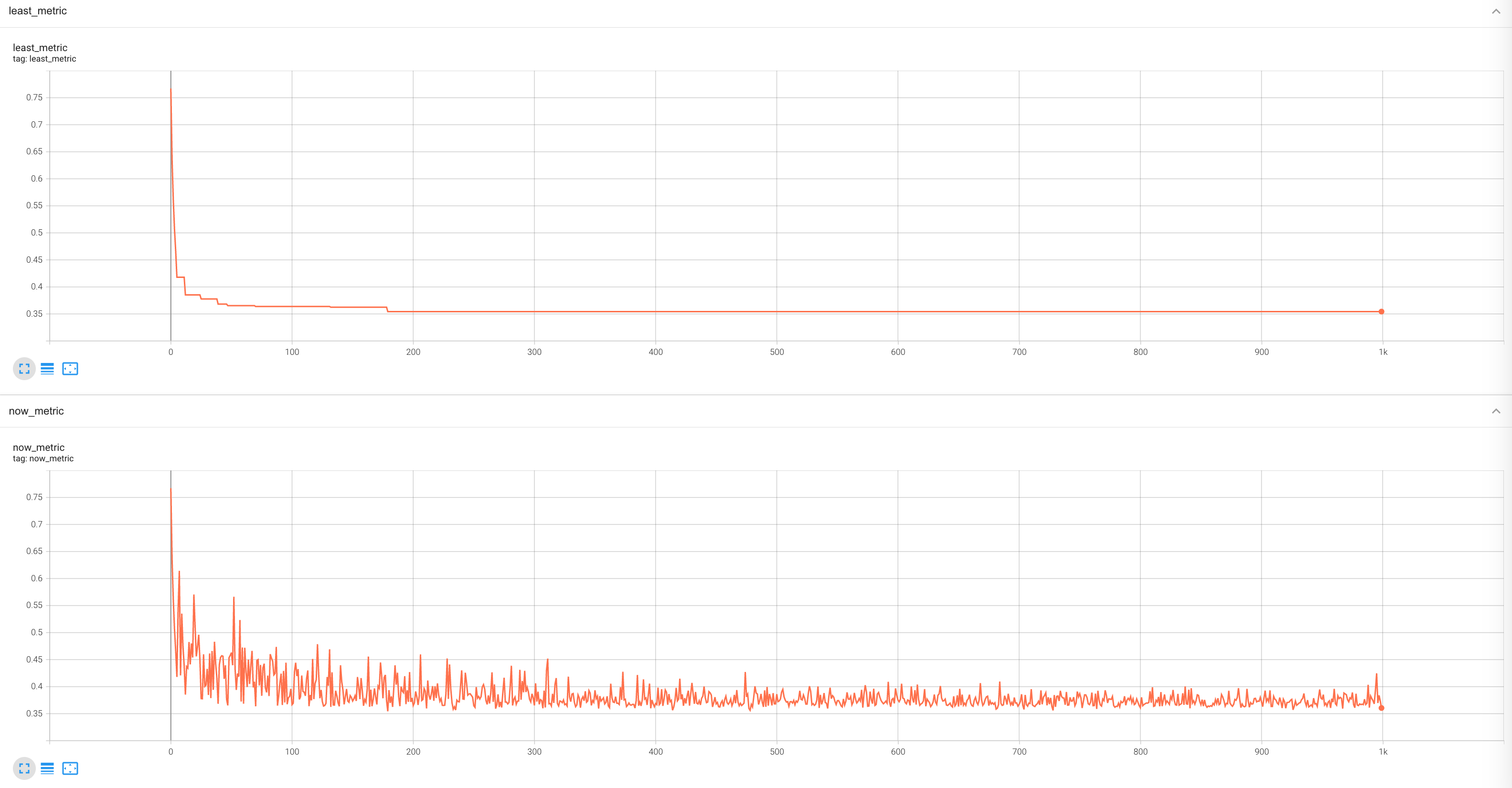
As shown in the figure above, among the various metrics recorded in tensorboard, now_metric and least_metric are used to record venv_metric. In this subtask, venv_metric is set to mae.

now_metric records the values of mae for each training epoch.
least_metric records the smallest value of now_metric among all epochs prior to the current training epoch. Therefore, it can be regarded as the lower bound of the curve contour in the now_metric graph.
When least_metric becomes lower, REVIVE will save or replace the saved virtual environment model.

We can see that after reaching 200 epochs of training, least_metric has been updated with a lower value. At this point, REVIVE saves the network model for the current epoch. Since least_metric does not decrease further, REVIVE does not save a new model. We can manually stop the training of the virtual environment model at this point and proceed to the subsequent policy training.

Rollout Chart Interpretation¶

The rollout chart refers to a graph that displays the actions taken and rewards obtained by a robot or agent at different time steps when it is run according to a specific policy. This chart is used to evaluate the effectiveness of the policy in a specific environment and identify areas for improvement. In the rollout chart, the horizontal axis represents the time steps, while the vertical axis represents the changes in the state and actions of the robot or agent.

By observing the rollout chart, we can gain insights into the behavior of the robot or agent during its execution and the rewards it receives. If we observe poor performance at certain time steps or negative outcomes resulting from certain actions, we can consider adjusting the policy to achieve better results in future runs. The rollout chart helps us diagnose and assess the differences between the virtual environment and real data.

After learning the virtual environment using the REVIVE SDK, REVIVE replays the training data (i.e., the historical dataset collected from the real environment) based on the specified logic of the decision flow. Since this historical data is collected from real environmental scenarios, such a comparison indirectly assists users in judging the differences or similarities between the learned virtual environment model and the real-world scenario.

Tip

Users can also refer to the tutorial on using a trained model to load the virtual environment model and generate rollout charts that meet their customization needs.

Here, we take the example of the Pendulum task to further explain the rollout chart saved by REVIVE.

metadata:

   graph:
     actions:
       - states
     next_states:
       - states
       - actions

   columns:
     - obs_states_0:
       dim: states
       type: continuous
     - obs_states_1:
       dim: states
       type: continuous
     - obs_states_2:
       dim: states
       type: continuous
     - action:
       dim: actions
       type: continuous

In the Pendulum task, we have established the decision flow chart mentioned above. The states have three-dimensional data, and the actions have one-dimensional data. For more detailed data descriptions, please refer to the Using REVIVE SDK to Control Pendulum Motion.

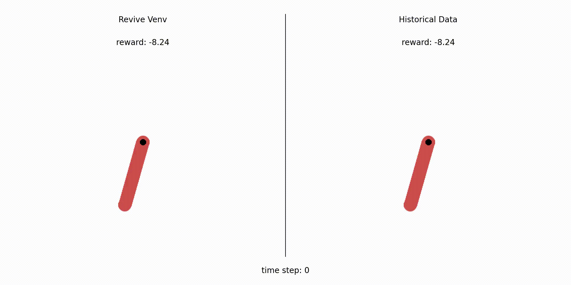
As shown in the animation above, the left side displays the motion of the pendulum in the REVIVE virtual environment, while the right side shows the motion of historical data in the real environment. We can understand the rollout chart saved by REVIVE as a two-dimensional line graph that compares the virtual environment model with the historical data sampled from the real environment, with the individual data dimension as the smallest unit.

REVIVE follows the following steps when generating the rollout chart:

REVIVE randomly samples 10 trajectories from the dataset for comparison between the virtual environment model and the real historical data. (REVIVE will trim these 10 randomly sampled trajectories to have the same length based on the shortest trajectory length in the training dataset).
REVIVE iterates over the data based on the names of nodes in the decision flow graph graph (refer to Decision Flow Graph and Array Data). The rollout chart is generated using this autoregressive method. Therefore, the rollout results are entirely based on the virtual environment model.
In the current example, REVIVE reads the node information from the graph and generates the rollout chart for the two nodes, actions and next_states, as well as the input node states. Therefore, the corresponding rollout charts are saved under the rollout_images directory based on the names of these three nodes.

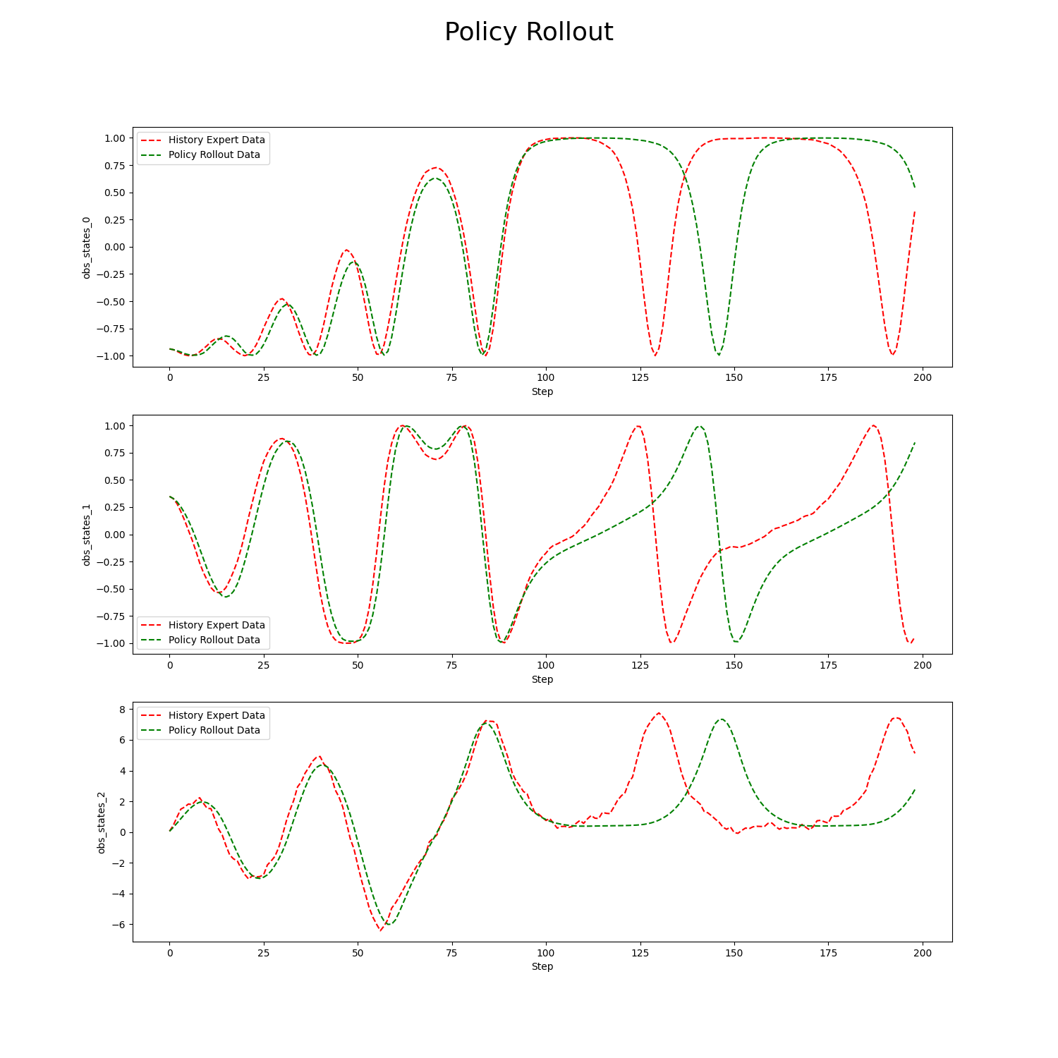
The above is an example of the rollout data for the states in the task Control Pendulum’s Movement Using REVIVE SDK.

The red dashed line represented by History Expert Data indicates the historical data used for training the virtual environment.
The red dashed line represented by Policy Expert Data indicates the historical data used for training the virtual environment.

Since states have three dimensions, the rollout data for each dimension is shown in the graph using the names defined in the decision flow’s columns as the y-axis labels. The x-axis represents the number of rollout steps, totaling 200 steps. This is also the length of each trajectory in the dataset.

From the graph, we can see that the autoregressive results of the virtual environment model closely resemble the real data with minimal error when the number of steps is less than 100. However, after surpassing 100 steps, although the virtual environment model can generate similar numerical trends, it still exhibits significant deviations from the real data. Therefore, when training the policy model based on this virtual environment, we should not set policy_horizon to a value greater than 100.

In conclusion, examining the rollout graph is the most intuitive way to assess the differences between the virtual environment model and the real environment (historical data). Through this method, we can roughly evaluate the degree of error in the virtual environment model in the shortest possible time, and use it as a basis for setting the policy_horizon step size in subsequent policy model learning. Although the virtual environment model cannot replicate the real environment with 100% accuracy, the presence of some errors does not mean that REVIVE cannot be used for policy optimization.