Prepare Data
Before using REVIVE SDK, you need to prepare your task data. The decision flowchart, training data, and reward function form a complete input for training tasks. The reward function is only required when training the policy model. In this section, we will first explain how to construct the decision flowchart file and training data file. You can also refer to the specific task scenarios in the Task Example section for a better understanding.
The decision flowchart and training data are closely coupled, with the decision flowchart storing the definition and relationship of the data, and the training data storing the corresponding node data:
REVIVE SDK uses a
.yamlfile to store the decision flowchart, which describes the relationship between the data.REVIVE SDK uses a
.npzor.h5file to store node data.
Write *.yaml file
The most important step in using the REVIVE SDK is to build the decision flowchart. The decision flowchart is a directed acyclic graph used to describe the interaction logic of business data. Each node in the decision flowchart represents data, and each edge represents a mapping relationship between data. The decision flowchart can be extended with any number of nodes as needed, and the order between nodes can be arbitrarily specified, with a single node serving as input to multiple nodes. The decision flowchart is stored in a .yaml file upon completion of construction.
A well-designed decision flowchart is an essential part of the REVIVE SDK, which can make training models more efficient and prediction results more accurate.
The .yaml file mainly includes two attributes. The graph describes the relationship
between each key node in the data;
the detailed description in columns indicates the property of each dimension of the data.
Generally speaking, you should define a decision flow (graph) before preparing the training data.
A .yaml file consists of three parts as follows:
Attribute |
Description |
|---|---|
graph |
the decision flow of all the agents in the real environment |
columns |
attribute description of the feature dimension |
In the *.yaml file, one can also include expert_function and other tools for using REVIVE.
An example description .yaml file is as follows:
metadata:

   graph:
     action:
     - obs
     next_obs:
     - obs
     - action

   columns:
     - obs_1:
         type : continuous
         dim : obs
         min : 0
         max : 1
     - obs_2:
         type : discrete
         dim : obs
         max : 15
         min : 0
         num : 16
     - action1:
         type : category
         dim : action
         values : [0, 1, 3]

   ...

   expert_functions:
     next_obs:
       'node_function' : 'dynamics.transition'
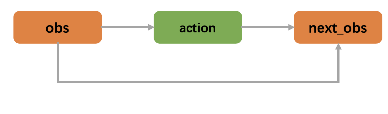
The first part of the yaml file, the graph, describes the constructed decision flow chart. For example, in the decision flow chart described in the above yaml file, there are three nodes in the graph: obs, action and next_obs. The “obs” node is the input for the action node, while the next_obs node takes both the obs node and the action node as inputs. This decision flow process conforms to real-world business logic: an agent makes actions based on observations (obs), and the environment transitions according to the current state (obs) and the agent’s actions (action).
A real-world task example is an autonomous driving car. The nodes in the decision flow chart can represent various sensors of the car, such as cameras, lidars, millimeter-wave radars, etc., which continuously gather information about the vehicle’s surroundings and transmit this information to the agent. In this case, the obs node can represent environmental information around the vehicle and the vehicle’s state information, such as the width and length of the road, speed limits, traffic signs, and the positions of other vehicles. The action node can represent the agent’s actions based on observations, such as acceleration, deceleration, turning, or stopping. The next_obs node can represent the new environmental information and the new state information of the vehicle after the agent has completed an action. When making decisions, the agent may calculate the optimal action for the next step based on the current observation result (obs) and the predicted environmental changes (action). The next_obs node will then contain new environmental information and new vehicle state information, which are obtained through the combined input of the obs node and the action node. Therefore, the information in the next_obs node is the result of the joint action of the inputs of the obs node and the action node, including the new environmental information around the vehicle and the new state information of the vehicle.
The decision flow chart describes how an agent makes decisions in a real-world environment. Each node can have multiple inputs, meaning that multiple node variables affect the output of the node. Each node in the decision flow chart represents a decision process used to calculate node variables, and the edges represent the flow of data. Since the variable names and decision relationships are completely variable, you should build a decision flow chart that conforms to the business logic based on specific task requirements.
The operational example of the decision flow chart corresponding to the above .yaml file is shown in the following figure. First, the obs node outputs data to the action node, and then the next_obs node uses the data from the obs and action nodes to calculate the value of the next_obs node.
Every key represents a decision node of the decision flow, like action and next_obs in the .yaml.
Key means the corresponding decision node is the output node in the decision flow. For example, action is the output node with input data from obs,
next_obs is the output node with input data from obs together with action.
The decision flow will be called recursively through state transition, for example, the value of next_obs at time step t will be passed to obs at time step t+1
And in the next iteration step, next_obs will be treated as obs.
The following animation describes how REVIVE recursively calls the decision flow.
The decision flowchart is a process that runs in a loop across multiple time steps. At each time step, the decision flowchart runs completely. During this process, the next_* nodes are treated as transition nodes, and their corresponding data will be used as input for the * nodes in the next time step. For example, the next_obs node data at time step t will be used as the obs node data at time step t+1. The following animation shows how the REVIVE SDK performs a looped call of the decision flowchart over time steps.
Important
“next_” must be the prefix for the state transitions defined by users, as these five characters are the only index for REVIVE to automatically search state transitions.
A decision flowchart can have multiple transition nodes, such as the next_o and next_s transition nodes in the following yaml decision flowchart.
graph:
   a:
   - o
   - s
   next_o:
   - o
   - a
   next_s:
   - o
   - s
   - a
Each node in the decision flow could get input data from more than one node, but would only compute the output bounded to itself.
Important
The graph is a DAG (Directed Acyclic Graph) in which there should contain at least one transition variable.
The second part of the yaml file describes the feature dimensions and their attributes in the format of a dictionary list. You should define the name and properties of each dimension of the node data. Each key of the dictionary represents the name of the feature dimension (e.g., obs_1), dim represents the node name to which the feature belongs (e.g., obs represents the feature belongs to the obs node), and type represents the type of feature data.
The REVIVE SDK supports the following three data types:
continuous: The continuous type indicates that the value of the feature can vary in a continuous real space. For example, the speed of a car is a continuous feature value. Users can also provide the
maxandminparameters to specify the range of values. If the user does not provide a value range, the minimum and maximum values will be automatically extracted from the training data for setting.discrete: The discrete type indicates that the feature value can only be selected from a set of discrete real numbers, and these real values have equal intervals within a given range. For example, age can be discretized into several age groups, such as 20-29 years old, 30-39 years old, etc. In this case, the discrete set can be
{20, 30, 40}. The max and min parameters specify the value range (they will be included in the discrete set). If the user does not provide a value range, the minimum and maximum values will be automatically extracted from the training data for setting. Users need to specify thenumparameter to limit the number of discretizations. In the above example, the valid values of the second dimension of obs are[0, 1, 2, ..., 15].category: The category data indicates that the value of the feature can only take a limited integer subset, and there is no numerical relationship between the numbers in the subset. For example, consider a person’s occupation type, which may belong to one of several occupation types, such as doctors, teachers, engineers, etc. This data type can be regarded as a category. Users need to specify category-like parameters to describe the values corresponding to each category. In the above example, the valid values of
actionare[0, 1, 3].
Note
The REVIVE SDK does not support data types in string format.
In the *.yaml file, we can also insert expert_function to import expert functions as expert knowledge to replace the learning of neural networks. Proper use of expert functions can reduce task difficulty and improve model training efficiency. For details, please refer to the section in :doc:` Advanced Tools <expert_function>`.
Note
By default, the first node of the decision flow chart is selected as the target policy node (the node to be optimized when training the policy). We can also use the -tpn parameter to specify the node we need as the policy node. For more details, please refer to train model.
Constructing Array Data
After writing the .yaml file, the user should construct the corresponding array data for the historical data according to the decision flow chart. The data should be a Python dictionary, with the node name as the key and the data of the Numpy array as the value. All values should be a 2D ndarray, with the sample size N as the first dimension and the number of features C as the second dimension. The key should correspond to the node name described in the graph of the .yaml file.
index:
indexis additional data used to mark the end index of each trajectory in the data. For example, if the data has a shape of (100, F) and contains two trajectories with lengths of 40 and 60, respectively,indexshould be set tonp.ndarray([40, 100]).
Once the data has been constructed as a dictionary, it should be stored in a single .npz or .h5 file. (.npz files can be saved using the numpy.savez_compressed function, while .h5 files can be saved using the revive.utils.common_utils.save_h5 function).
import numpy as np
from revive.utils.common_utils import save_h5

data = { "obs": obs_array, "act": act_array, "index": index_array}
# save npz file
np.savez_compressed("data.npz", **data)
# save h5 file
save_h5("data.h5", data)
Validation Data (Optional)
In addition, we can provide another data file as a validation dataset. The dataset should have the same data structure as the training file, which means that both files can be described using the same .yaml file.
If this data is not provided, the REVIVE SDK will automatically split the training data into two parts in a 1:1 ratio and use them as the training and validation datasets. We can modify the relevant parameters in the configuration file to control the ratio and method of data splitting.
This section describes how to construct a dataset that can be used by the REVIVE SDK, including building decision flow graphs and describing the feature dimensions and properties of the data. The decision flow graph is a directed acyclic graph that represents the interaction logic between business data, and can be freely extended according to task requirements. The constructed decision flow graph and array data should be stored in .yaml and .npz files, respectively. The REVIVE SDK provides some runnable examples, including decision flow graphs and array data that are already prepared, which can be used as a reference to deepen your understanding.
Here are some examples of the REVIVE SDK: